This is an addendum to my poster presentation at MSJ-SI 2014 "Hyperbolic Geometry and Geometric Group Theory". The poster is available here. This page is intended to exhibit pictures that I couldn't include in the poster.
Throughout this article, we assume that \(S\) is a once-punctured torus.
Basics
We fix a pair of generators \(\alpha\), \(\beta\) of \(\pi_1(S)\) so that their commutator \([\alpha, \beta]\) is peripheral. We define the \(\mathrm{SL}(2,\mathbb{C})\)-character variety by
where two representations are equivalent if they are conjugate. This has a structure of an affine algebraic set, and there is an isomorphism of the varieties
defined by
The \(\mathrm{PSL}(2,\mathbb{C})\)-character variety \(X(S)\) is defined similarly. It is known that \(X(S)\) is isomorphic to the quotient of \(X_{SL}(S)\) by the action of \((\mathbb{Z}/2\mathbb{Z})^2\) generated by \((x,y,z) \mapsto (-x,y,-z)\) and \((x,y,z) \mapsto (x,-y,-z)\).
For a positive real number \(l\), we define the linear slice \(X(l)\) as a subvariety of \(X(S)\) defined by the equation \(x = 2 \cosh (l/2)\). In other words, \(X(l)\) is the set of representations whose complex lengths of \(\alpha\) are equal to \(l\). The complex Fenchel-Nielsen coordinates for \(X(l)\) gives a bijection from \(\{ \tau \in \mathbb{C} \mid -\pi < \mathrm{Im}(\tau) \leq \pi\}\) to \(X(l)\) defined by
Pictures of quasi-Fuchsian representations
We let \(QF(S)\) be a subset of \(X(S)\) consisting of faithful representations with quasi-Fuchsian images. We let \(QF(l) = QF(S) \cap X(l)\) . Our main interest in this article is the shape of \(QF(l)\) in \(X(l)\). We show some experimental pictures of \(QF(l)\) (indicated by shaded regions) in \(X(l)\).
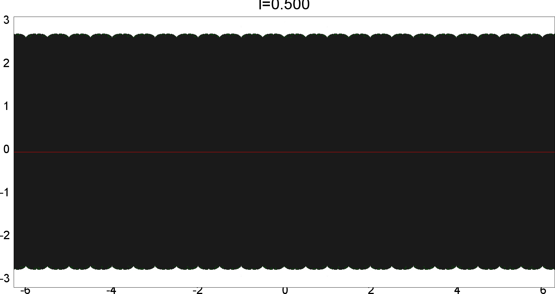
l=0.50
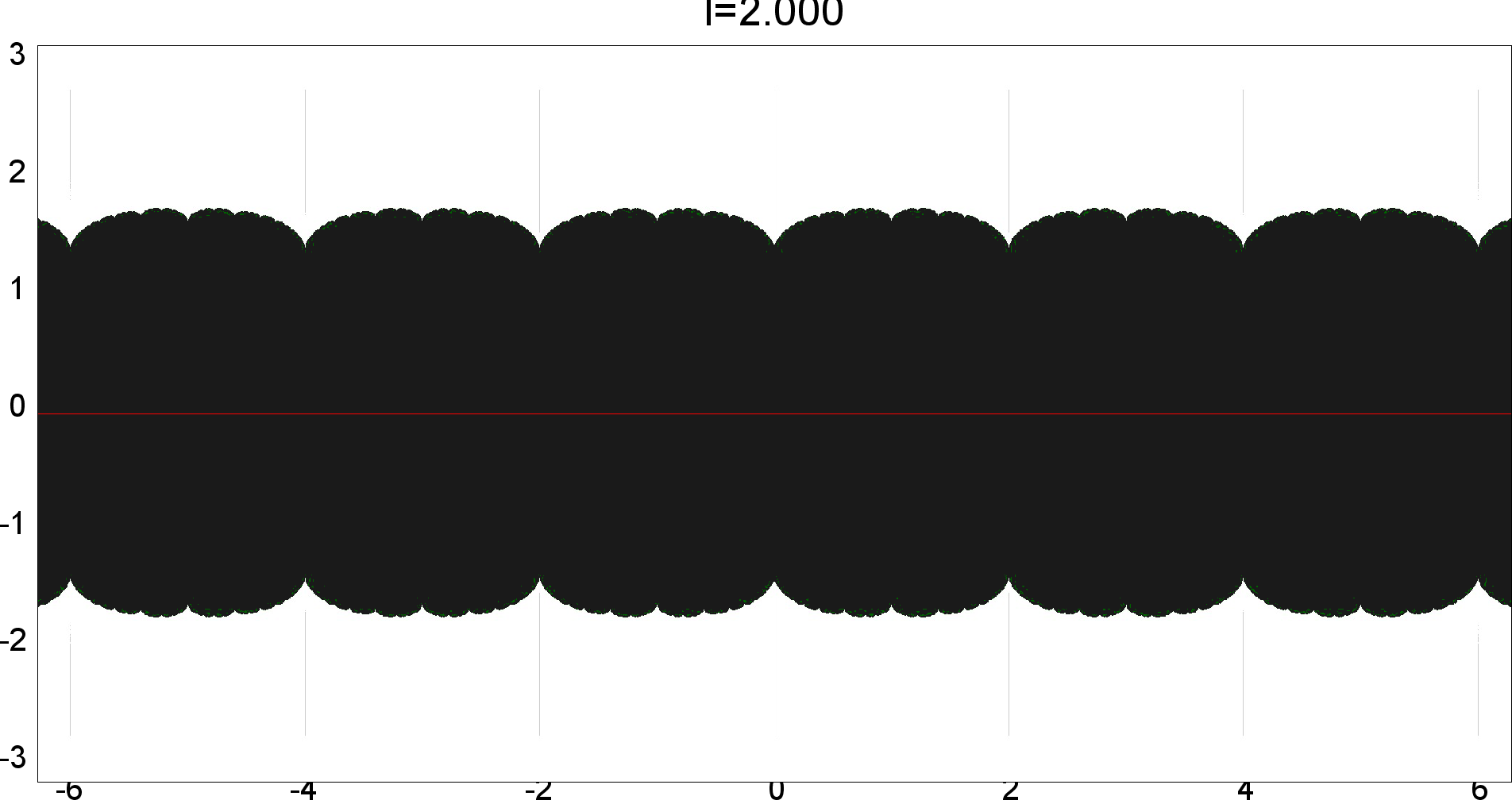
l=2.00
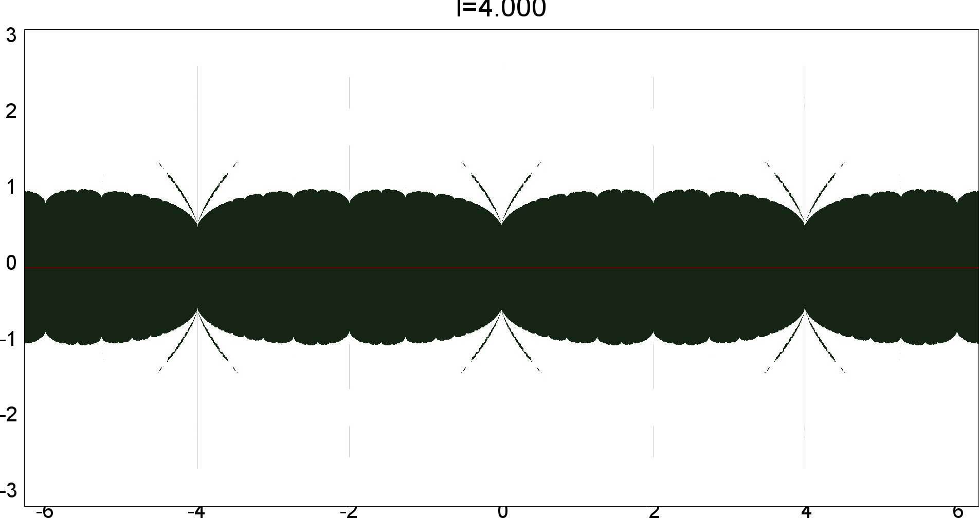
l=4.00
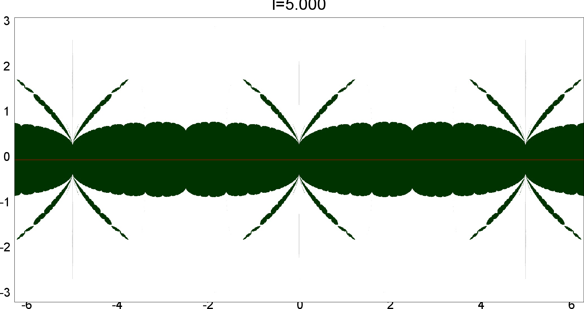
l=5.00
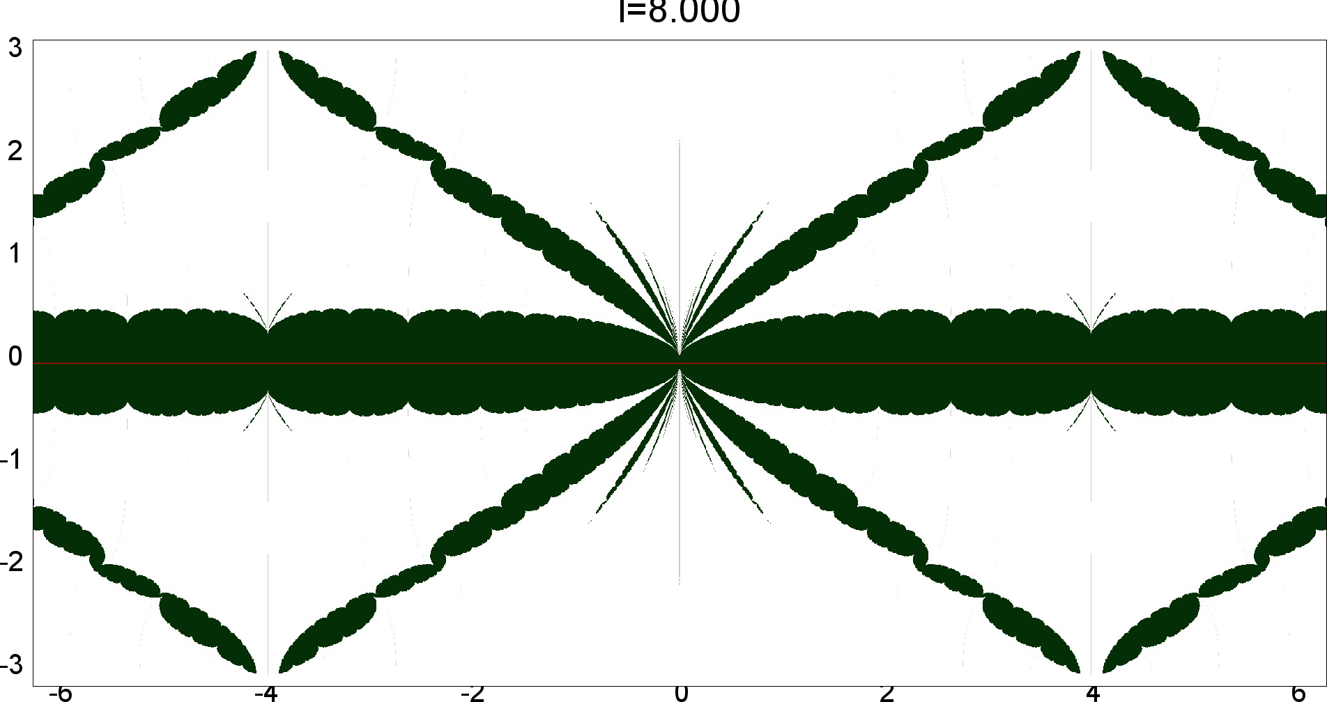
l=8.00
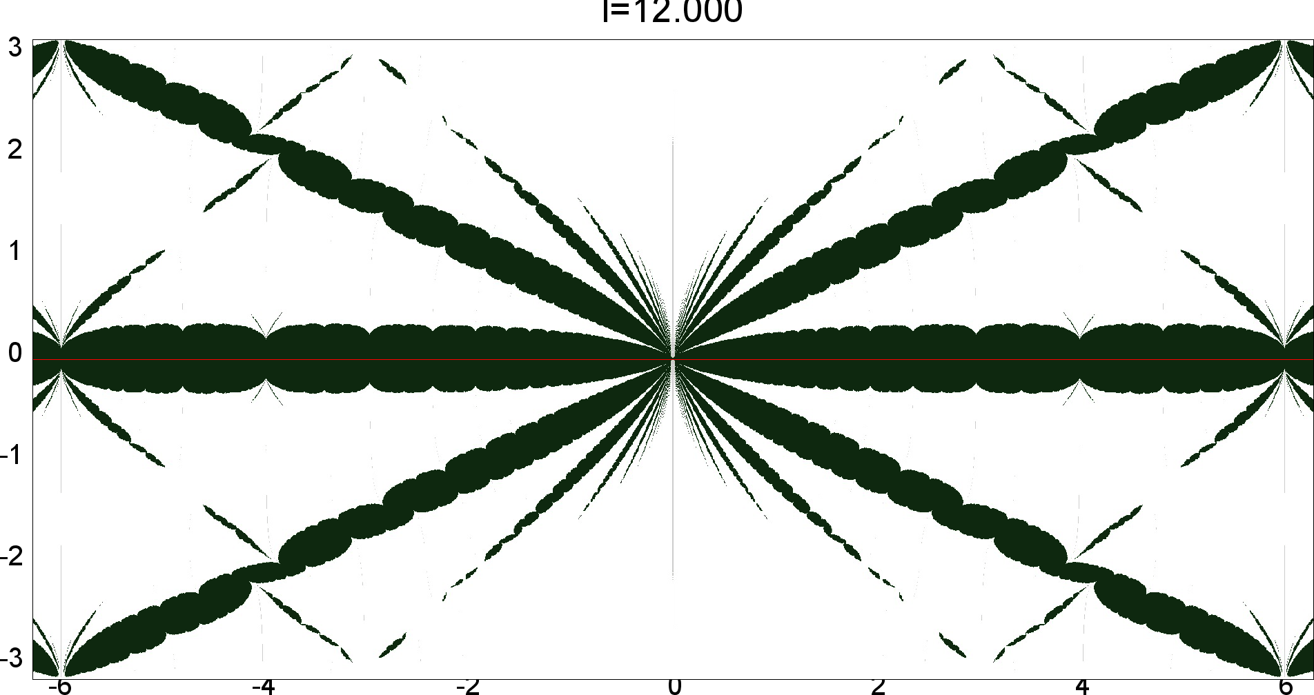
l=12.00
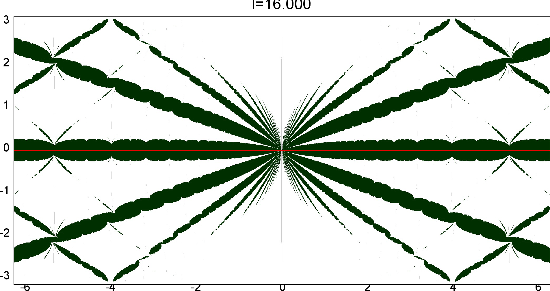
l=16.00
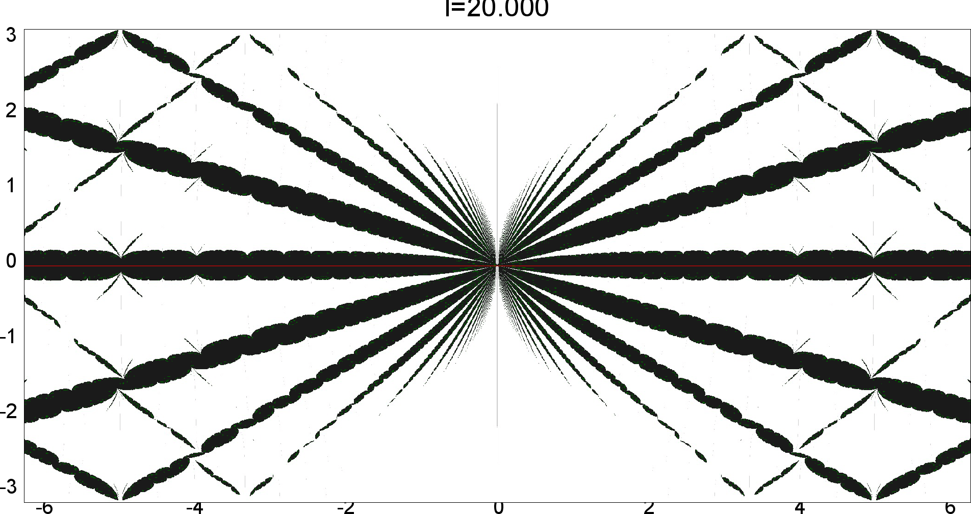
l=20.00
(These pictures are drawn by a program plotting the points satisfying BQ-conditions (Bowditch's Q-conditions), which are conjectually and well-confirmed experimentally (at least type-preserving case) equivalent to the condition that the corresponding representation is quasi-Fuchsian. I thank Yasushi Yamashita for sharing his program.)
As the pictures suggest, the number of components increases as \(l\) is getting longer. Here we list some known facts.
- The real line corresponds to the Fuchsian representations. In particular, \(QF(l)\) contains the real line.
- \(QF(l)\) is a union of disks. (A consequence of the disk convexity of \(QF(S)\) by C. McMullen.)
- If \(l\) is sufficiently small, \(QF(l)\) has only one component. (Otal)
- The Dehn twist along \(\alpha\) acts on \(X(l)\) as \(\tau \mapsto \tau + l\), thus \(QF(l)\) is invariant under this translation.
From the last fact with a few extra observations, we can show that, if \(QF(l)\) has a component not containing Fuchsian representations, there are infinitely many. Even after taking the quotient by the action \(\tau \mapsto \tau + l\), we can show that \(QF(l)\) has arbitrary large number of components if \(l\) is sufficiently long. Moreover, non-locally connectedness properties shown by Bromberg imply that it may have infinitely many components in the quotient. We observe these phenomena in pictures near `cusp points' (the representations the curve \(\beta\) cusped).
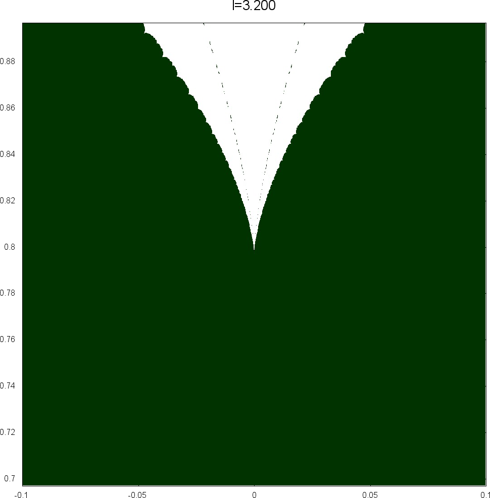
l=3.20
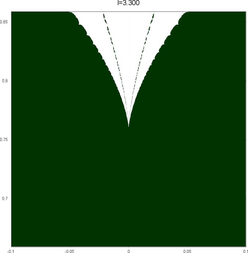
l=3.30
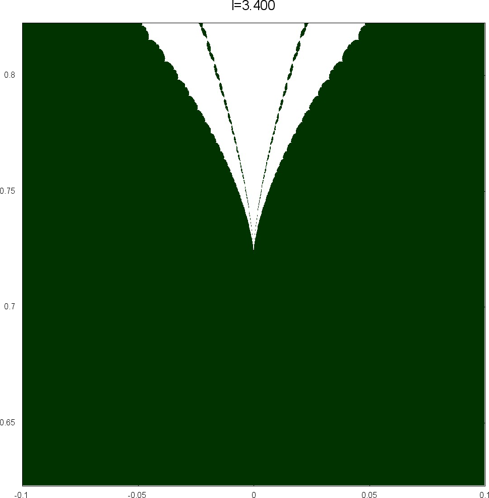
l=3.40
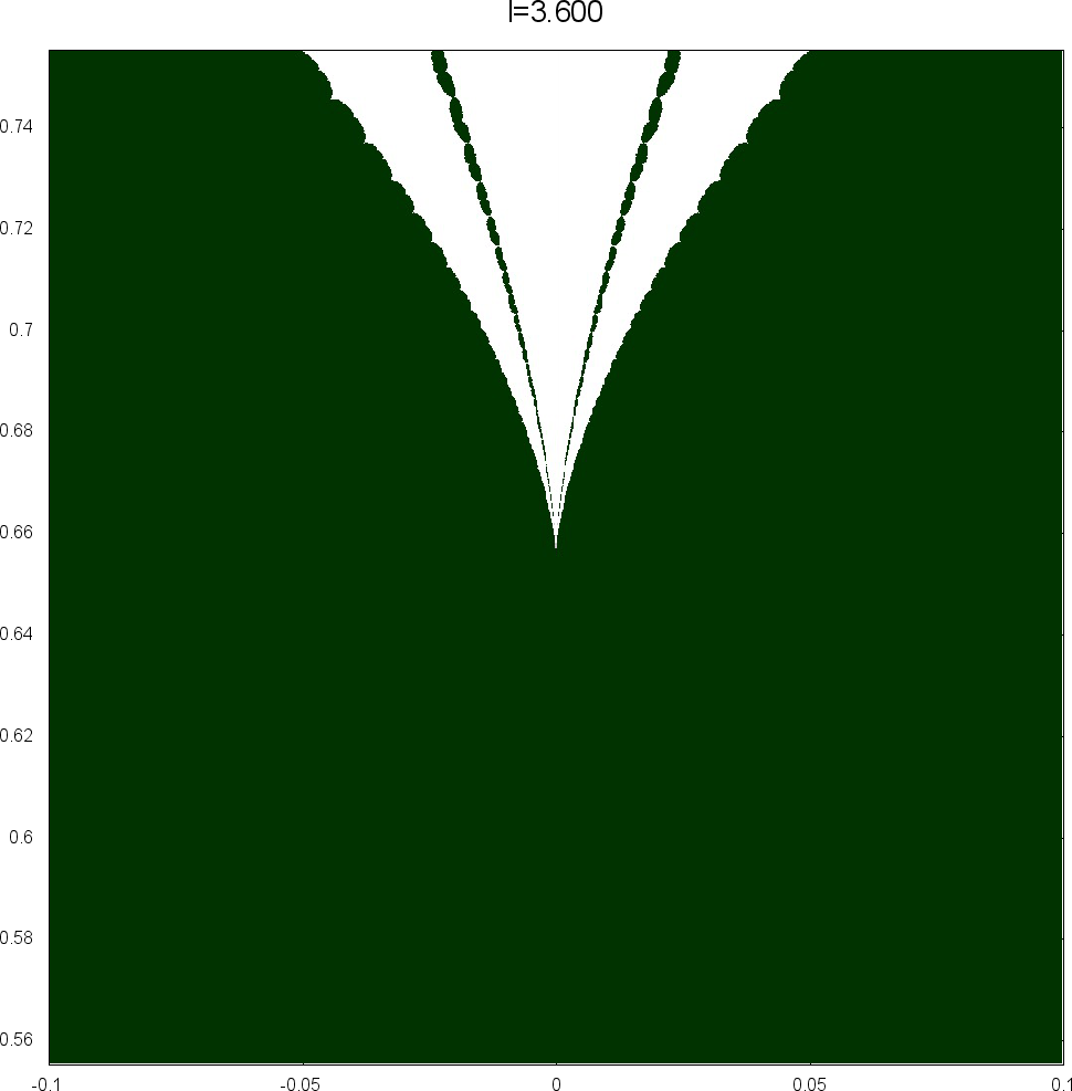
l=3.60
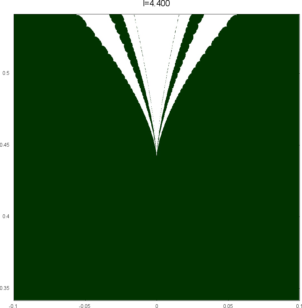
l=4.40

l=4.50

l=4.60

l=4.70
Complex projective structures and grafting
A complex projective structure is a geometric structure locally modeled on \(\mathbb{C}P^1\). In terms of \((G,X)\)-structure, this is a \((\mathrm{PSL}(2,\mathbb{C}), \mathbb{C}P^1)\)-structure. If a surface has a complex projective structure, by analytic continuation of the local structure, we obtain a representation, called the holonomy, and an equivariant map from the universal cover of the surface to \(\mathbb{C}P^1\), called the developing map. In general, a \((G,X)\)-structure defines a holonomy (up to conjugation) and a developing map (up to precomposition by \(G\)), and conversely such pair determines the \((G,X)\)-structure uniquely.
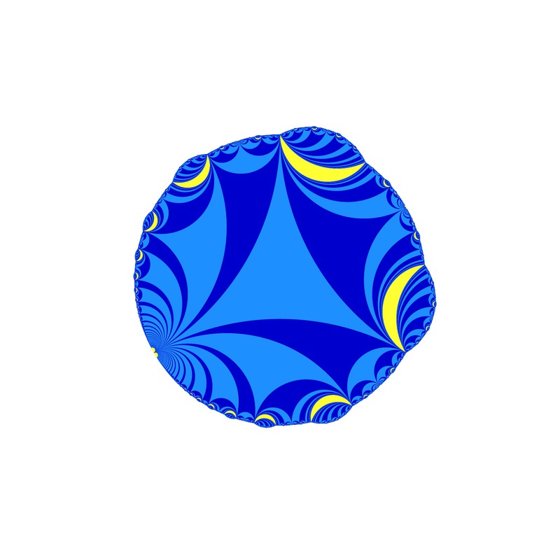
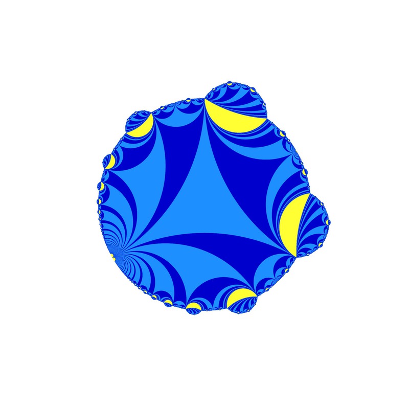
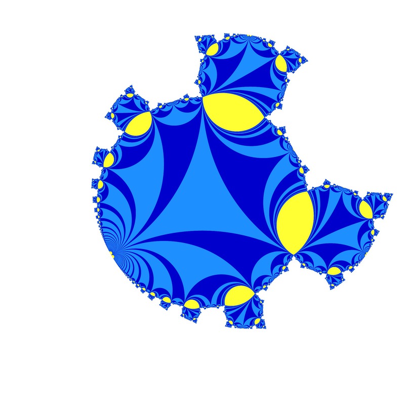
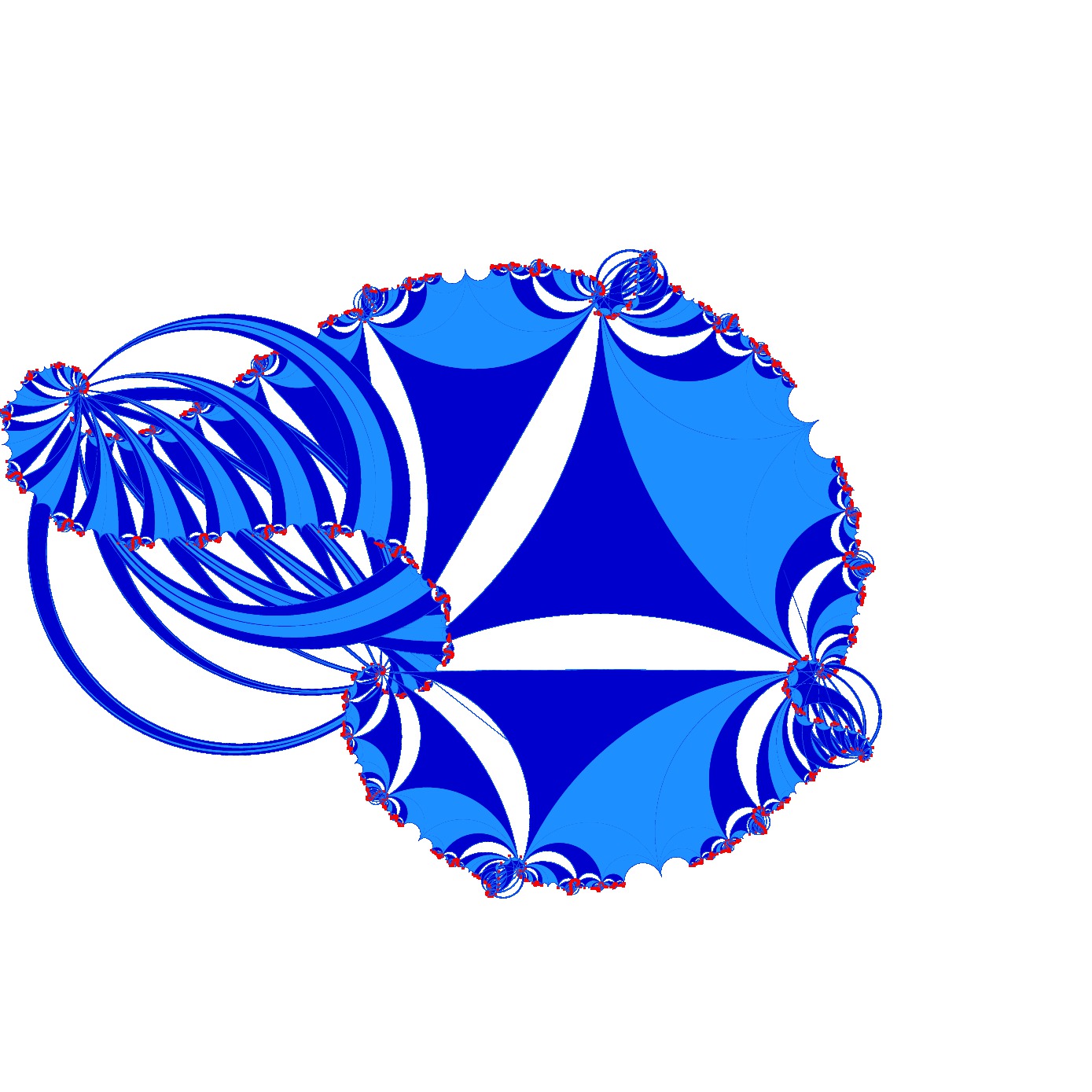
A Fuchsian uniformization gives a complex projective structure. We can construct a complex projective structure from a Fuchsian uniformization by inserting annulus along a simple closed geodesic. This operation is called the grafting. The followings are developing maps of some grafted surfaces. In these pictures, yellow strips are the lifts of the grafted annulus. (We will explain the parameters \(l, t, b\) later.)

l=1.0, t=0.050, b=0.000
l=1.0, t=0.050, b=0.500
l=1.0, t=0.050, b=1.000
l=1.0, t=0.40, b=2.000
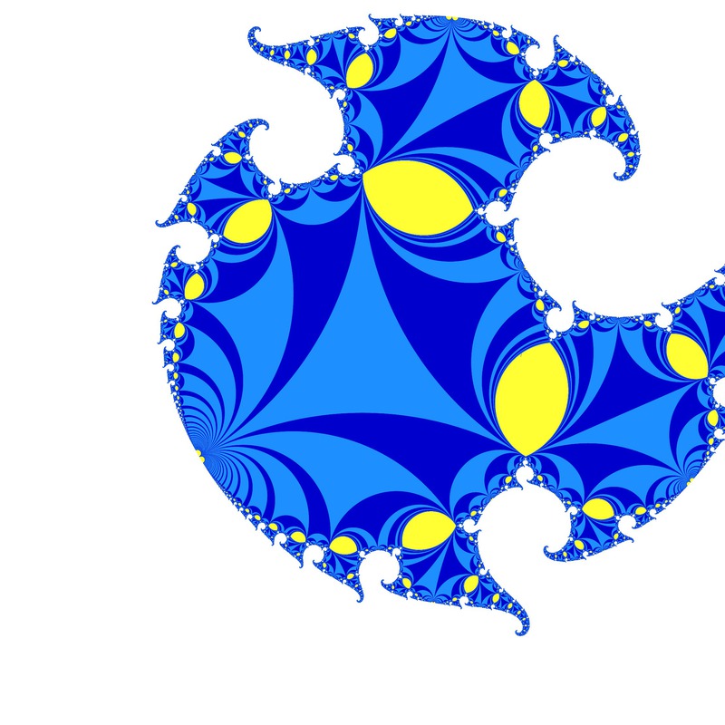
l=1.0, t=0.40, b=2.200

l=1.0, t=0.40, b=2.250
We can define \(P(S)\) the set of marked complex projective structures as in the case of Teichmüller space \(T(S)\). For a simple closed curve \(\gamma\) on \(S\), the grafting of an annulus of height \(b\) along \(\gamma\) gives a map \(\mathrm{Gr}_{b \cdot \gamma} : T(S) \to P(S)\).
Complex earthquakes
For a positive real number \(l\), let \(X_l\) be the marked hyperbolic surface such that the length of \(\alpha\) is equal to \(l\) and the geodesics homotopic to \(\alpha\) and \(\beta\) are orthogonal. (In fact, the surface is uniquely determined by these conditions.) Let \(\overline{\mathbb{H}} = \{ \tau \mid \mathrm{Im}(\tau) \geq 0\}\). The complex earthquake for \(\alpha\) is a map \(\overline{\mathbb{H}} \to P(S)\) defined by
\[ \tau = t + b \sqrt{-1} \mapsto \mathrm{Gr}_{b \cdot \alpha}(\mathrm{tw}_{t \cdot \alpha}(X_l)), \]where \(\mathrm{tw}_{t \cdot \alpha} : T(S) \to T(S)\) is the Fenchel-Nielsen twisting of distance \(t\) along \(\alpha\). The holonomy gives a map \(\mathrm{hol} : P(S) \to X(S)\), which is known to be a local homeomorphism. By composting \(\mathrm{hol}\) with the complex earthquake, we obtain a map \(\overline{\mathbb{H}} \to X(S)\). We can check that the range of this map is \(X(l)\), and it coincides with the complex Fenchel-Nielsen coordinates for \(X(l)\) modulo \(2 \pi \sqrt{-1} \mathbb{Z}\). Thus a complex earthquake is regarded as a lift of the complex Fenchel-Nielsen coordinates.
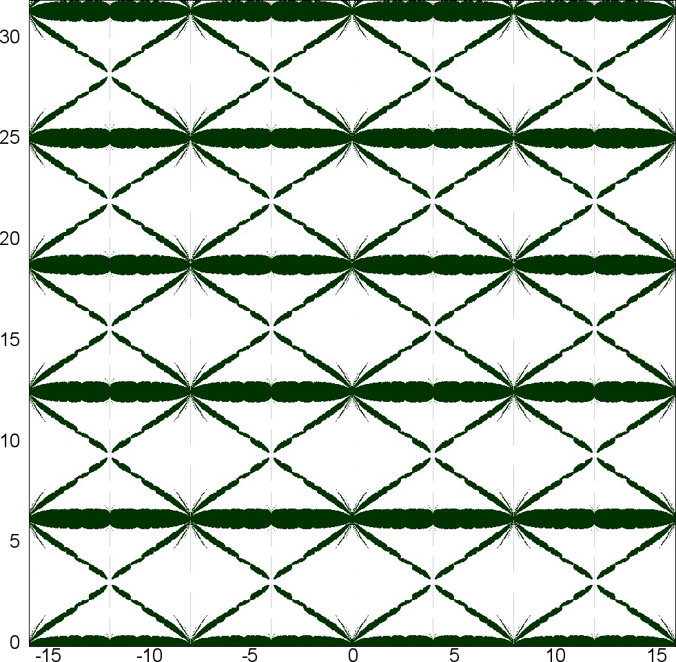
l=8.0
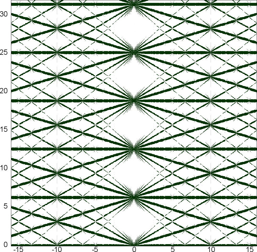
l=20.0
Exotic components
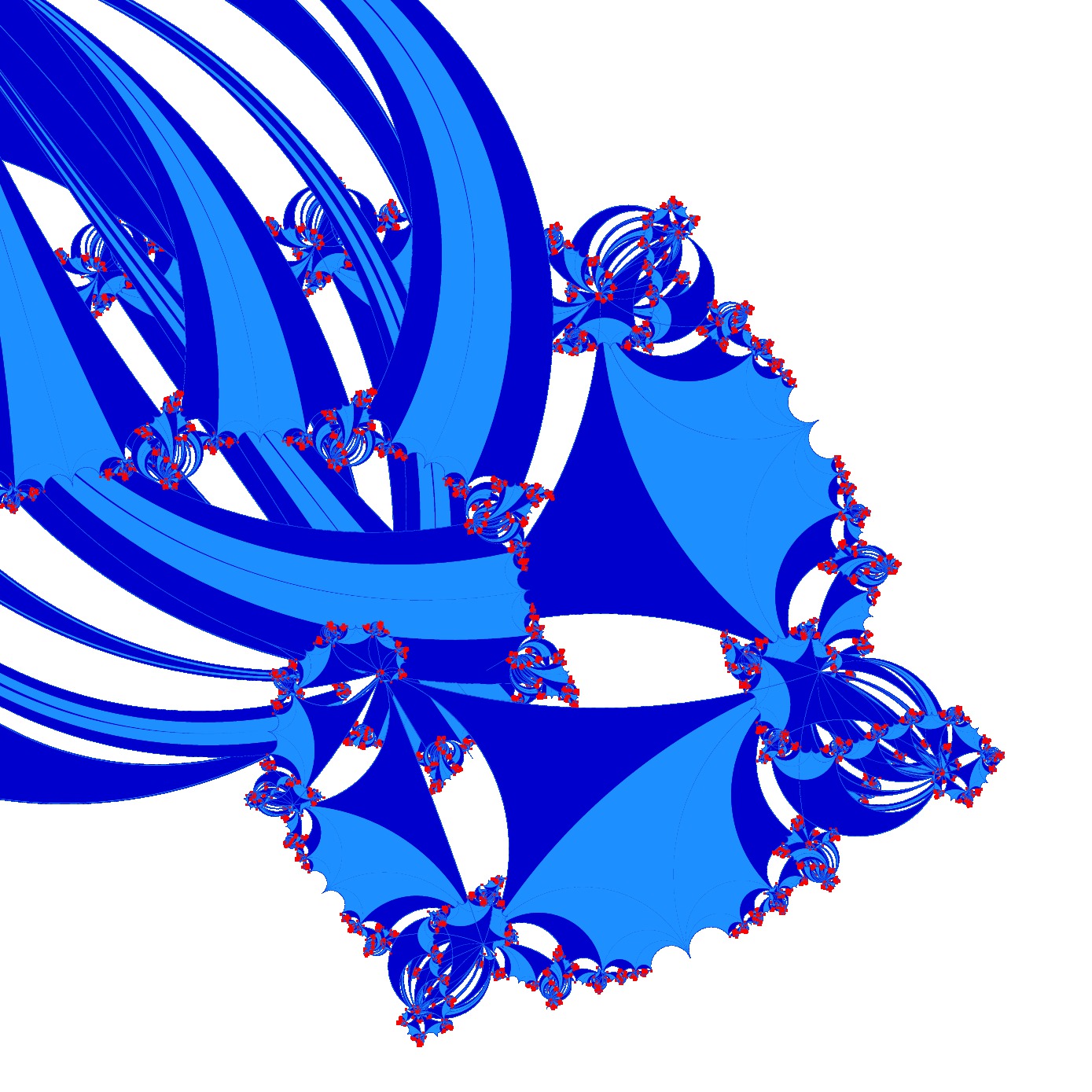
Since the image of a complex earthquake is in \(P(S)\), each point in the image corresponds to a complex projective structure. We give some pictures of the developing maps of complex projective structures in the image of a complex earthquake.
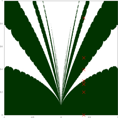
The complex earthquake for l=8.0 near the origin.
l=8.0, t=0.40, b=0.000

l=8.0, t=0.40, b=0.200
l=8.0, t=0.40, b=0.270
l=8.0, t=0.40, b=0.298
l=8.0, t=0.40, b=0.398
l=8.0, t=0.40, b=0.500
l=8.0, t=0.40, b=0.850
We remark that the last three pictures (b=0.398, 0.500, 0.850) are INCORRECT. Since the correct developing maps are far from embedding, so they were too mixed to visualize. I don't know the reason why, but if we turn some of triangles (colored blue or light-blue) `inside-out', pictures become relatively simple.
From these pictures, we can observe that components not containing the real line correspond to exotic projective structures, i.e. complex projective structures with non-injective developing maps. Actually, we can show that the existence of exotic projective structure in the complex earthquake (except integral multiple of \(2\pi\alpha\)) implies that \(QF(l)\) has more than one component.
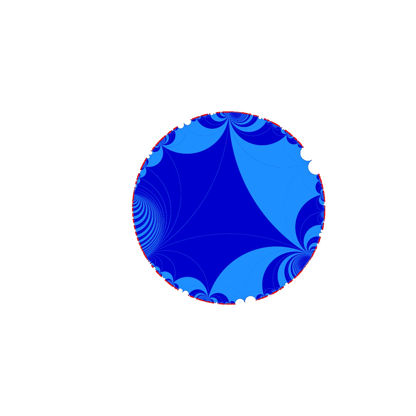
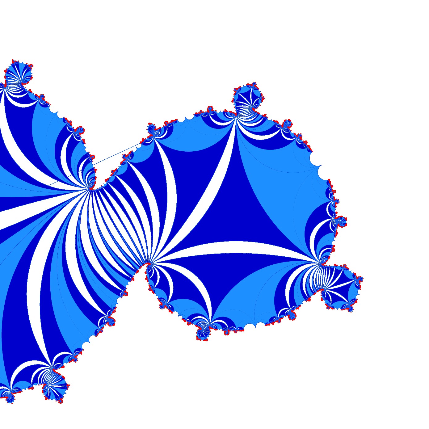
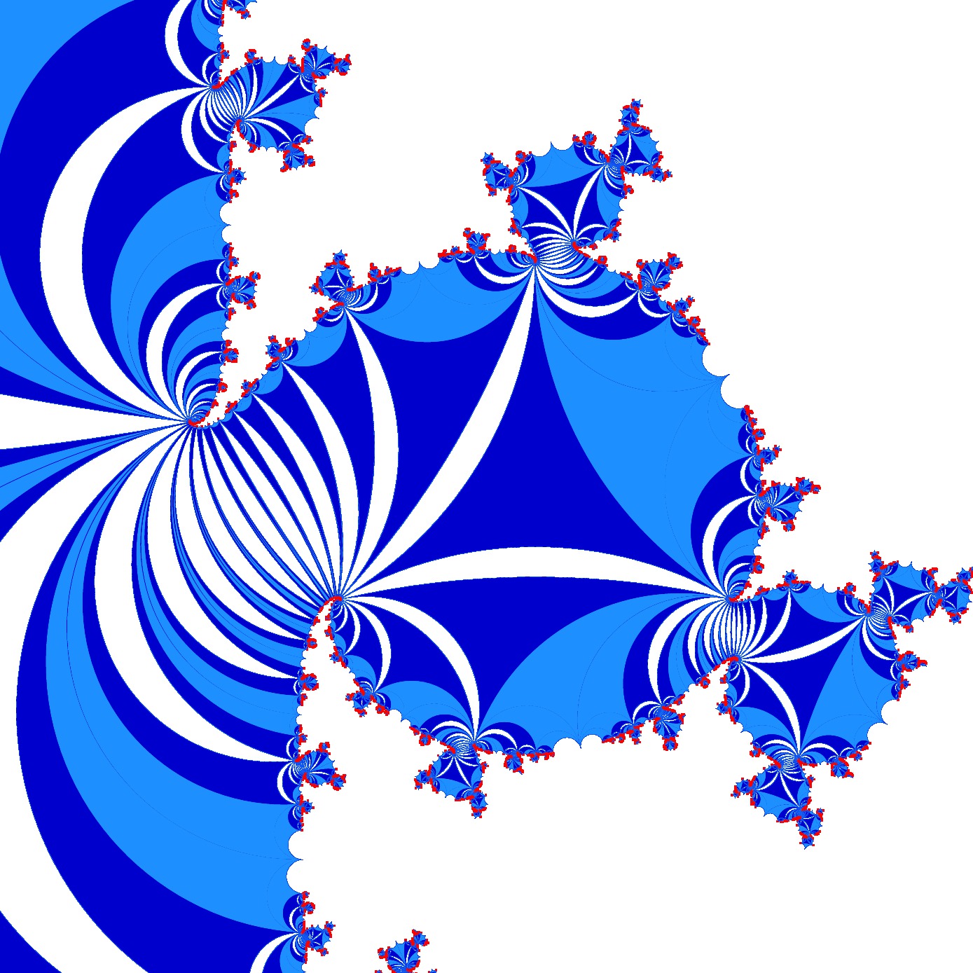
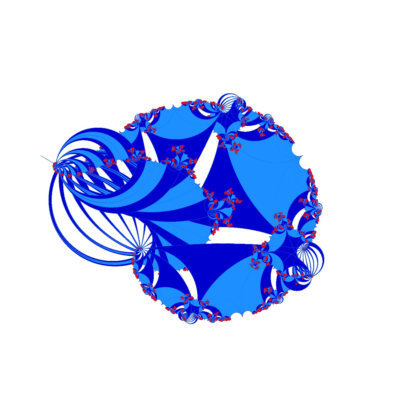
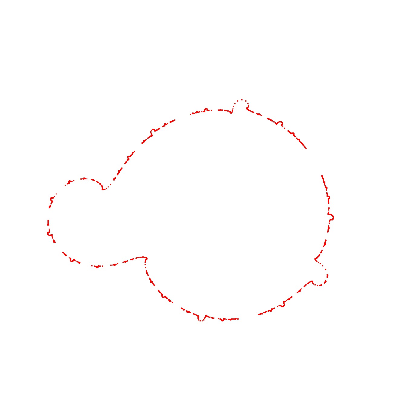
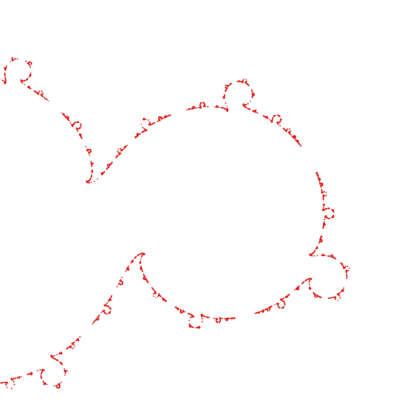
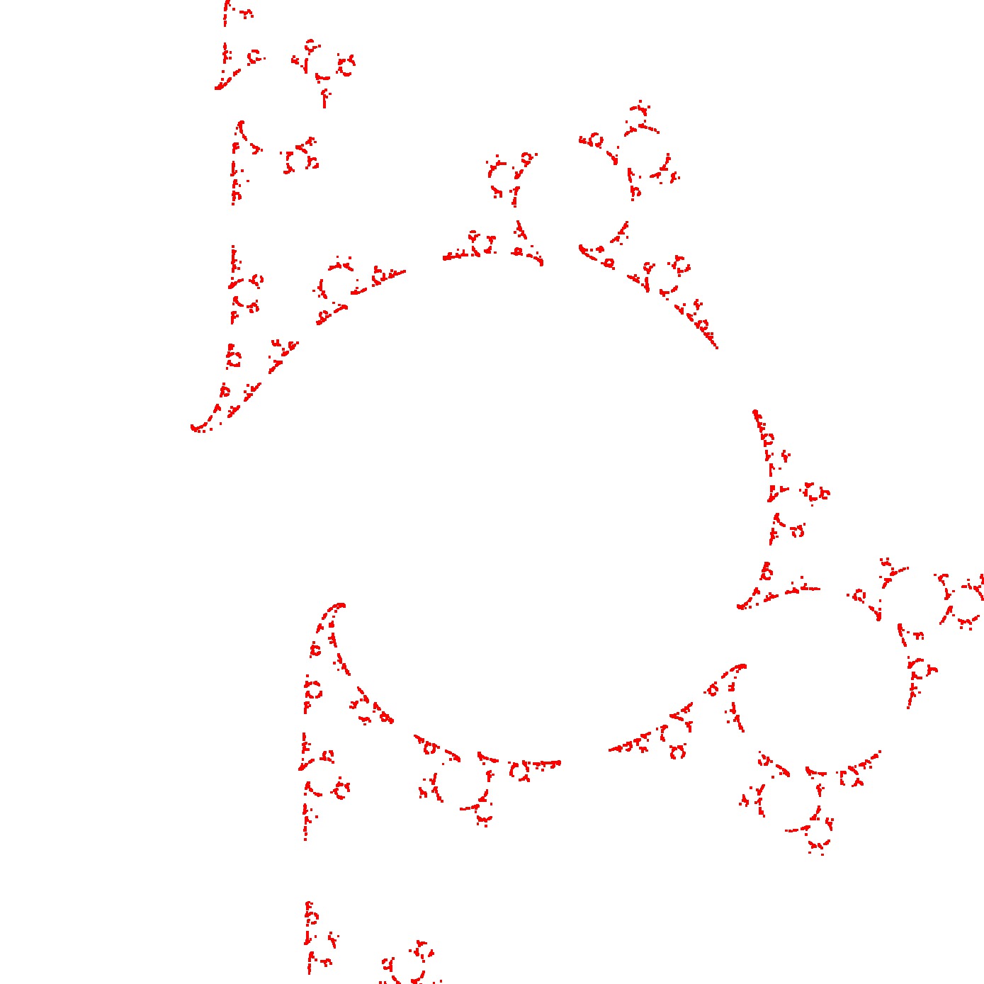
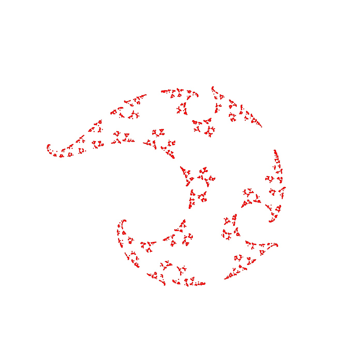
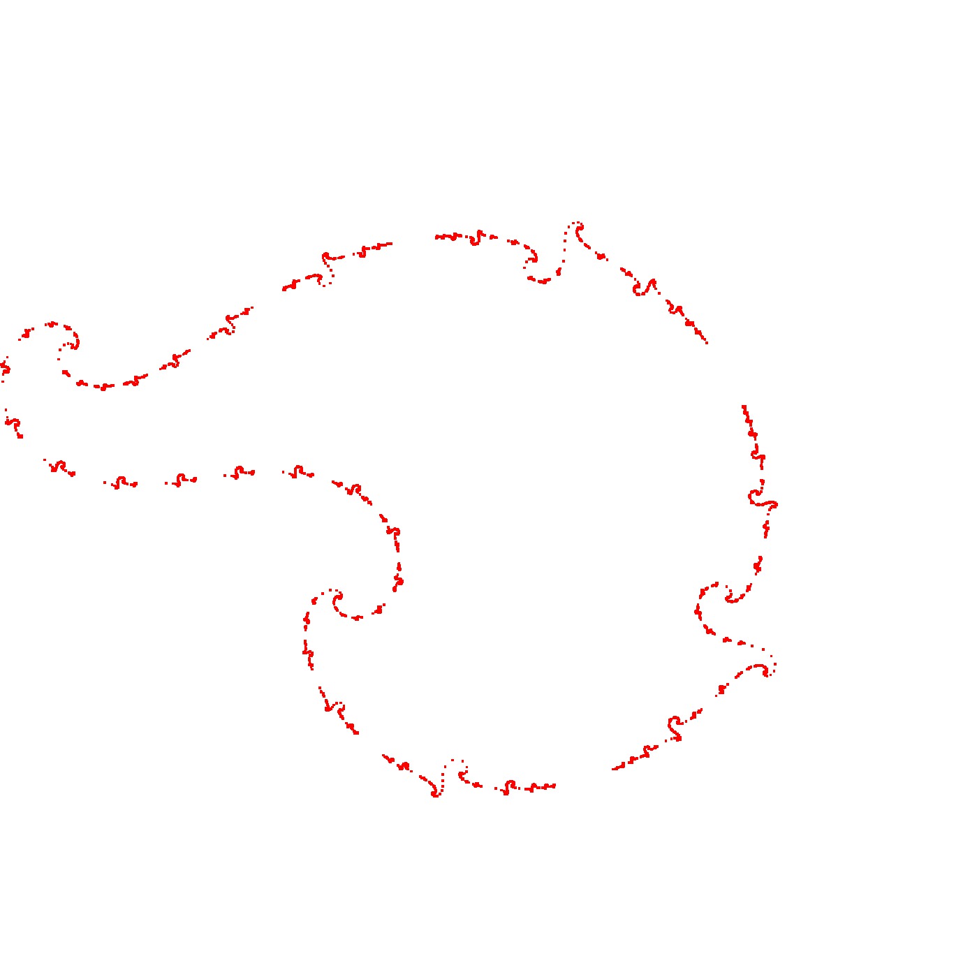
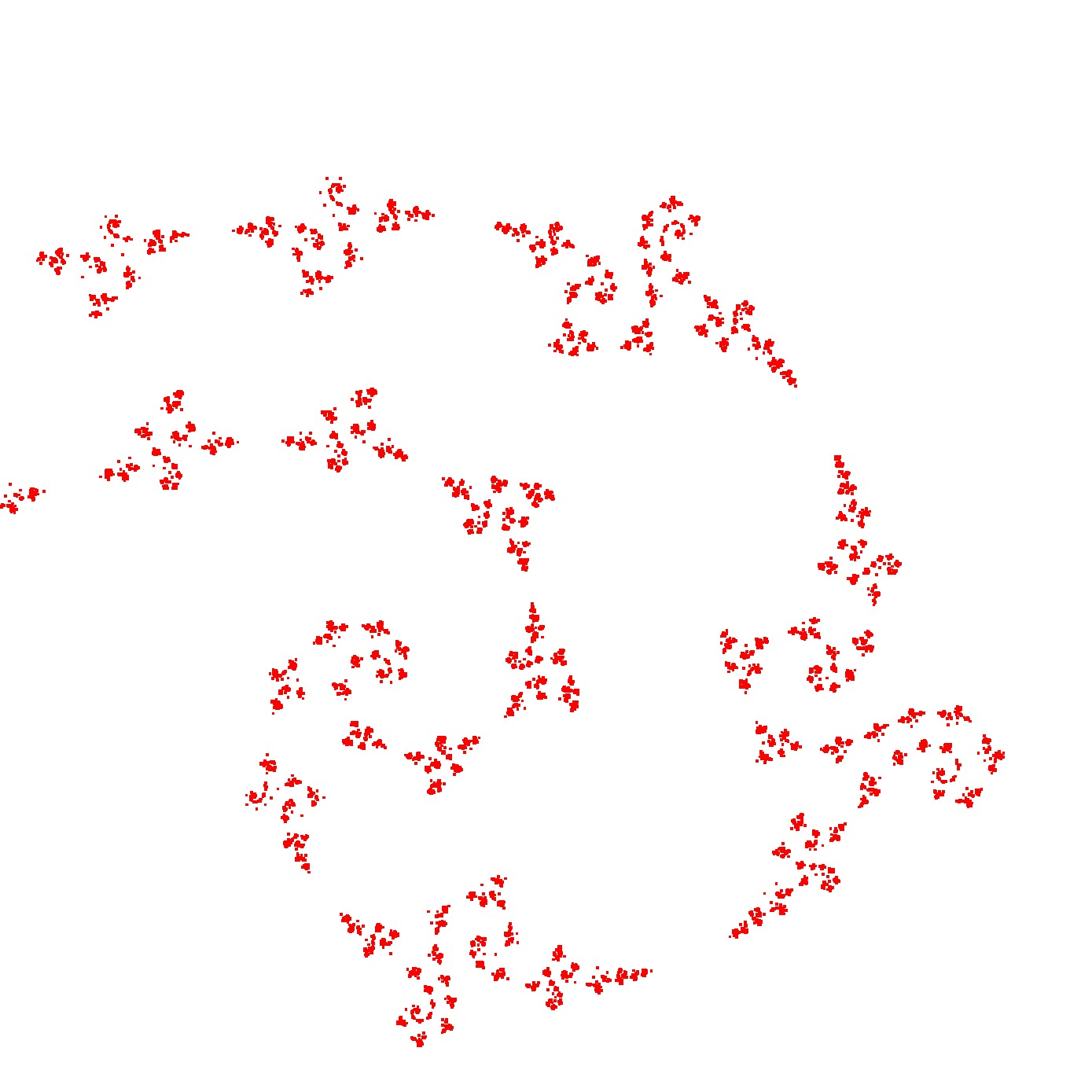
Lastly, we show the limit sets corresponding to the above developing maps.
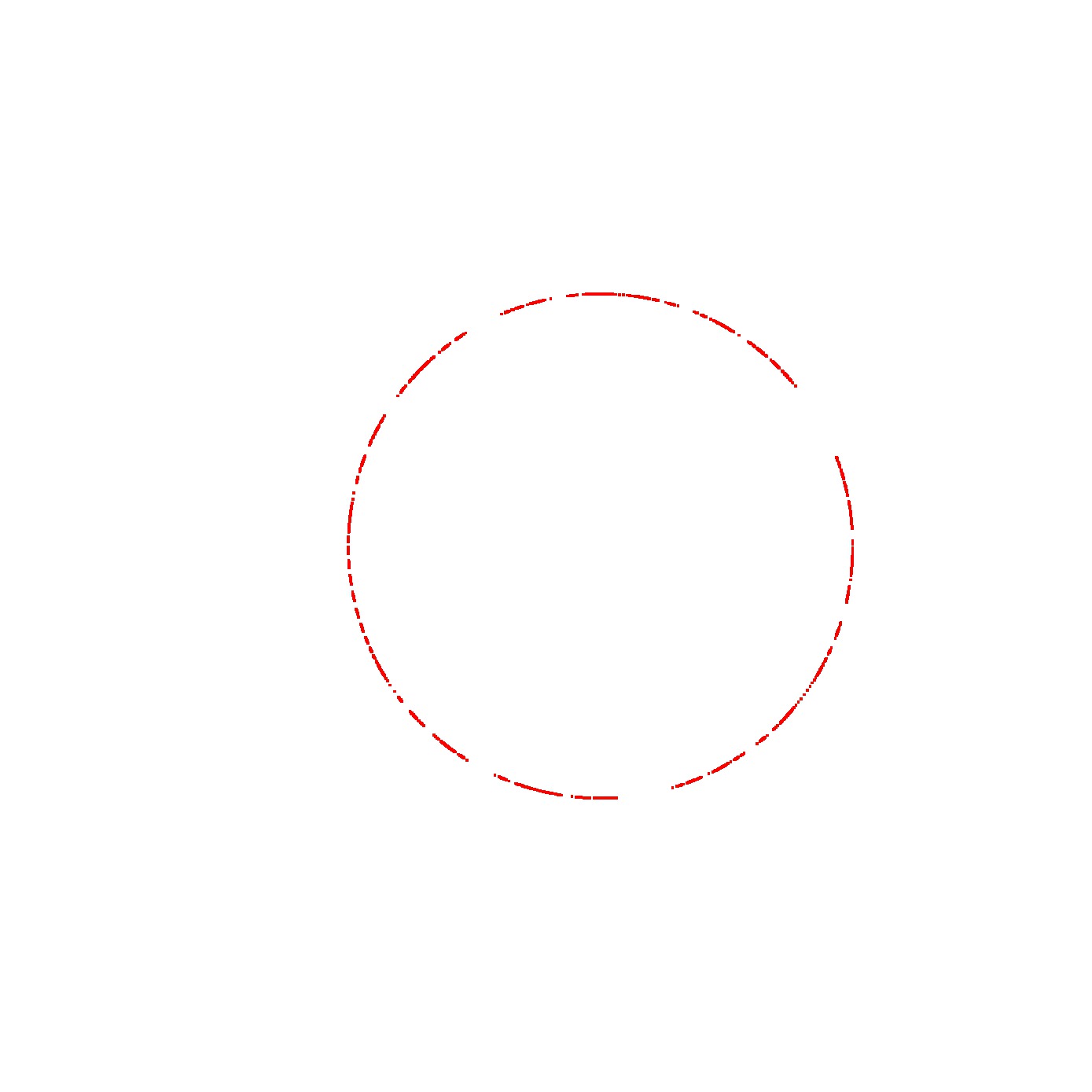
l=8.0, t=0.40, b=0.000
l=8.0, t=0.40, b=0.200
l=8.0, t=0.40, b=0.270
l=8.0, t=0.40, b=0.298
l=8.0, t=0.40, b=0.398
l=8.0, t=0.40, b=0.500
l=8.0, t=0.40, b=0.850